Plot behavior on boundaries

Plot behavior on boundaries with and without well images

plot_bounds_behavior(wells, aquifer, length.out = 100)

Arguments

wells	wells object with each row containing rate Q [m^3/s], diam [m], radius of influence R [m], & coordinates x [m], y [m]
aquifer	Afuifer object containing aquifer_type, h0, Ksat, bounds, z0 (for confined case only)
length.out	The number of points to evaluate on each boundary

Value

Two ggplot objects that show behavior on the boundaries, one for head and one for flow

Examples

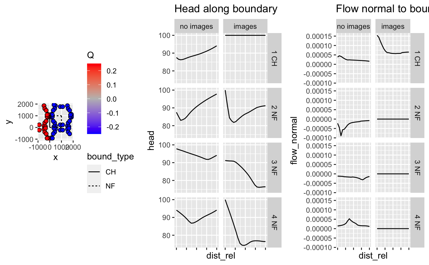
aquifer <- aquifer_confined_example
wells <- generate_image_wells(define_wells(wells_example), aquifer)
gg_list <- plot_bounds_behavior(wells,aquifer,length.out=20)

library(ggplot2)
p_domain <- ggplot() +
  geom_point(data=wells,aes(x,y,fill=Q),color="black",size=2,shape=21) +
  scale_fill_gradient2(low="blue",high="red",mid="gray") +
  geom_segment(data=aquifer$bounds,aes(x1,y1,xend=x2,yend=y2,linetype=bound_type)) +
  coord_equal()
gridExtra::grid.arrange(p_domain,gg_list$p_h,gg_list$p_f,nrow=1)
gg_list$table
#> # A tibble: 4 x 5
#>   bound `Mean flow, imag… `Mean flow, no im… `Mean head, imag… `Mean head, no i…
#>   <chr>             <dbl>              <dbl>             <dbl>             <dbl>
#> 1 1 CH          0.0000762          0.0000254             100                89.4
#> 2 2 NF          0                  0.0000260              87.9              90.4
#> 3 3 NF          0                  0.0000185              84.1              94.4
#> 4 4 NF          0                  0.0000234              80.7              90.5
gg_list$bounds_behavior
#> # A tibble: 160 x 15
#>        x     y   bID  dist dist_rel x_unit_norm y_unit_norm  head  flow_x
#>    <dbl> <dbl> <int> <dbl>    <dbl>       <dbl>       <dbl> <dbl>   <dbl>
#>  1     0 1000      1   0     0                1           0  87.5 3.86e-5
#>  2     0  947.     1  52.6   0.0526           1           0  86.5 4.54e-5
#>  3     0  895.     1 105.    0.105            1           0  86.2 4.22e-5
#>  4     0  842.     1 158.    0.158            1           0  86.4 3.63e-5
#>  5     0  789.     1 211.    0.211            1           0  86.8 3.03e-5
#>  6     0  737.     1 263.    0.263            1           0  87.3 2.59e-5
#>  7     0  684.     1 316.    0.316            1           0  87.7 2.32e-5
#>  8     0  632.     1 368.    0.368            1           0  88.1 2.36e-5
#>  9     0  579.     1 421.    0.421            1           0  88.5 2.30e-5
#> 10     0  526.     1 474.    0.474            1           0  88.8 2.26e-5
#> # … with 150 more rows, and 6 more variables: flow_y <dbl>, flow_normal <dbl>,
#> #   flow_mag <dbl>, bound_type <chr>, im <fct>, BT <chr>