anem-vignette
Gopal Penny
2020-07-23
anem-vignette.RmdThis package was created to evaluate the hydraulic relationships among wells, in order to estimate the effect of a group of wells on drawdown at these wells or other wells. It it based on method of images from the analytical element modeling approach, in which the 2-dimensional characteristics of aquifers are reproduced by strategically placing wells within the domain.
This package models simple aquifer and well configurations. The boundaries of the aquifer can be specified as no flow or constant head boundaries, and the corners of the aquifer must be right angles. For fully bounded aquifers, this means that the aquifer must be a rectangle. The constant head boundaries take the head of the undisturbed aquifer, h0.
Units are designed for length dimensions given in meters (or m2), and time in seconds.
As you will see in this vignette, the package has a number of functions that are used to set up the aquifer boundaries and wells. For practical purposes, the package was designed for simple but real aquifers, and wells and boundaries of the aquifers can be imported as shapefiles and then prepared. The basic functionality of the package, described in more detail in sections below, can be seen in the following figure.

- Aquifer scenario with four wells and arrows indicating constant background flow towards the river. (b) Well images and radii of influence for bottom-right well (red). (c) Reproduction of the no-flow and constant-head boundaries for single well using well images. (d) Hydraulic head and flow field for scenario. Note that the stream, flowing from top to bottom, goes from gaining to losing.
Understanding the method of images
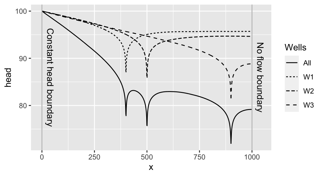
The package relies on the principle of superposition and the method of images to generate groundwater hydrodynamics, illustrated by the two figures below (see ?get_segments_behavior and ?get_stream_function, respectively, which give examples for generating similar plots). The principle of superposition states that, because the groundwater equations are linear, the solution to the equations can be calculated as the sum of solutions. In the example below, the drawdown of the water table is calculated as the sum of drawdown due to three individual wells.
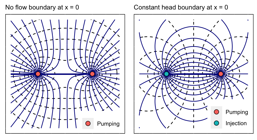
In the method of images, wells are mirrored across aquifer boundaries to reproduce characterics of the boundary, such as no flow or constant head. The following examples demonstrate (a) how a no-flow boundary is created by mirroring a well across the boundary, and (b) how a constant head boundary is recreated by mirroring the well and inverting the pumping.
A simple example of drawdown relationships
Load packages for the vignette
Aquifers in this package are characterized by:
- Aquifer type, confined or unconfined
- Saturated hydraulic conductivity, Ksat
- Resting hydraulic head, h0
- Thickness of the aquifer, z0 (confined aquifers only)
- Porosity of the aquifer, n
- Aquifer boundaries, characterized by:
- Boundary ID, or bID
- Coordinates in a cartesian plane, given as slope, m, and intercept, b, and coordinates (x1, y1, x2, y2)
- Boundary type, NF, CH, or PB
- Additional user-defined parameters
Use the define_aquifer() function to create a new aquifer, which has the class aquifer. This class is essentially a list with names parameters and a separate print method.
# define aquifer
bounds_df <- data.frame(bound_type=c("CH","NF","NF","NF"),m=c(Inf,0,Inf,0),b=c(0,1000,1000,0))
aquifer_unconfined <- define_aquifer("unconfined",1e-3,bounds=bounds_df,h0=100,n=0.35)
print(aquifer_unconfined)
#> # aquifer_type: unconfined
#> # Ksat: 0.001
#> # h0: 100
#> # n: 0.35
#> # bounds:
#> # A tibble: 4 x 8
#>     bID bound_type     m     b    x1    y1    x2    y2
#>   <int> <chr>      <dbl> <dbl> <dbl> <dbl> <dbl> <dbl>
#> 1     1 CH           Inf     0     0  1000     0     0
#> 2     2 NF             0  1000     0  1000  1000  1000
#> 3     3 NF           Inf  1000  1000  1000  1000     0
#> 4     4 NF             0     0     0     0  1000     0
#> # recharge (undisturbed water table):
#>     No recharge zones
Wells are characterized by:
- Well ID, or wID
- Location x, y
- Pumping rate (+ for injection, - for pumping), Q
- Radius of influence, R
- Diameter, diam
- Well images (which are noted in the
well_imagecolumn) - Additional user-defined columns, including groups or weights.
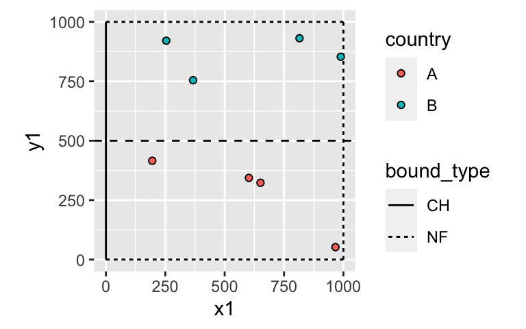
The code below Defines 8 pumping wells using random locations and arbitrarily divides wells into countries “A” and “B” using a threshold at y = 500 m. The define_wells() function ensures that the wells have all appropriate columns, and the class of the returned object is a tibble (which functions like a data.frame, but has a couple bells and whistles). Also note that the radius of influence (R) is defined arbitrarily, but there is also a function to calculate this manually – see ?get_ROI for more details.
The generate_image_wells() function generates well images to recreate the bounderies defined by the aquifer, aquifer_unconfined.
# define wells and well images
set.seed(15)
wells_actual <- define_wells(x = runif(8,0,1000),
                             y = c(runif(4,0,500),runif(4,500,1000)),
                             Q = -1/4,
                             diam = 1,
                             R = 1000,
                             weights = 1,
                             country = rep(c("A","B"),each=4))
wells <- wells_actual %>% generate_image_wells(aquifer_unconfined)
print(wells)
#> # A tibble: 68 x 11
#>      wID     Q     R  diam     x      y well_type well_image weights
#>    <dbl> <dbl> <dbl> <dbl> <dbl>  <dbl> <fct>     <chr>        <dbl>
#>  1     1 -0.25  1000     1  602.  344.  Pumping   Actual           1
#>  2     2 -0.25  1000     1  195.  416.  Pumping   Actual           1
#>  3     3 -0.25  1000     1  966.   52.3 Pumping   Actual           1
#>  4     4 -0.25  1000     1  651.  323.  Pumping   Actual           1
#>  5     5 -0.25  1000     1  367.  755.  Pumping   Actual           1
#>  6     6 -0.25  1000     1  989.  853.  Pumping   Actual           1
#>  7     7 -0.25  1000     1  815.  931.  Pumping   Actual           1
#>  8     8 -0.25  1000     1  254.  921.  Pumping   Actual           1
#>  9     9 -0.25  1000     1  602. 1656.  Pumping   Image (+Q)       1
#> 10    10 -0.25  1000     1  602. -344.  Pumping   Image (+Q)       1
#> # … with 58 more rows, and 2 more variables: country <chr>, orig_wID <int>
Plot the aquifer and wells.
ggplot() +
  geom_segment(data=aquifer_unconfined$bounds,aes(x1,y1,xend=x2,yend=y2,linetype=bound_type)) +
  geom_abline(slope=0,intercept=500,linetype="dashed") +
  geom_point(data=wells_actual,aes(x,y,fill=country),shape=21) +
  coord_equal()
Get drawdown relationships using get_drawdown_relationships(). This function calculates the average drawdown at wells in each group defined by the column group_column. The average is taken as the weighted mean, determined by the weights_column. The weights were previously set equal for all wells so that the result here is a simple mean. The results show PHIii and PHIij.
drawdown_relationships <- get_drawdown_relationships(wells, aquifer_unconfined, group_column=country, weights_column=weights)
drawdown_relationships
| var | pot | units | description |
|---|---|---|---|
| PHI_A_A | 1199.6188 | [m^2/cumec] | Weighted effect of pumping [cumec] in group A on discharge potential [m^2] in group A |
| PHI_A_B | 189.2822 | [m^2/cumec] | Weighted effect of pumping [cumec] in group B on discharge potential [m^2] in group A |
| PHI_B_A | 189.2822 | [m^2/cumec] | Weighted effect of pumping [cumec] in group A on discharge potential [m^2] in group B |
| PHI_B_B | 1342.9247 | [m^2/cumec] | Weighted effect of pumping [cumec] in group B on discharge potential [m^2] in group B |
Plot the head and flow
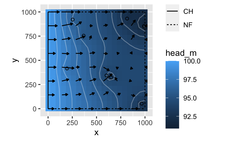
The hydrodynamics of the aquifer can be mapped by obtaining gridded heand flow using the get_gridded_hydrodynamics() function. The function takes as input the wells, aquifer, and grid dimensions for head and flow. It returns a list object with data.frames for head and flow, which can then be plotted.
gridded_1 <- get_gridded_hydrodynamics(wells,aquifer_unconfined,c(20,20),c(8,8))

ggplot() +
  geom_raster(data=gridded_1$head,aes(x,y,fill=head_m)) +
  geom_contour(data=gridded_1$head,aes(x,y,z=head_m),color="white",alpha=0.3) +
  geom_segment(data=gridded_1$flow,aes(x,y,xend=x2,yend=y2),
               arrow = arrow(ends="last",type="closed",length=unit(1,"mm")),color="black") +
  geom_segment(data=aquifer_unconfined$bounds,aes(x1,y1,xend=x2,yend=y2,linetype=bound_type)) +
  geom_point(data=wells %>% filter(wID==orig_wID),aes(x,y),shape=21) +
  coord_equal()
#> Warning: Removed 2 rows containing missing values (geom_segment).
Check the head and flow along the boundaries
The function get_bounds_behavior() is a helper function to generate hydraulic properties at the boundaries. It obtains hydraulic head and the flow normal to the boundaries by setting boundaries to segments and using get_segments_behavior(). Normal flow is defined such that positive flow has some component in the x-direction (the y-direction depends on the normal vector for the boundary). The function plot_bounds_behavior() is a wrapper around get_bounds_behavior(), and it can be used to quickly compare the hydraulic head along the boundaries and flow across the boundaries under two scenarios:
- no images (ie, homogeneous, uniform aquifer – all well images removed)
- images (ie, aquifer with boundaries – all well images intact)
bounds_behavior <- plot_bounds_behavior(wells,aquifer_unconfined)
gridExtra::grid.arrange(bounds_behavior$p_h,bounds_behavior$p_f,nrow=1)
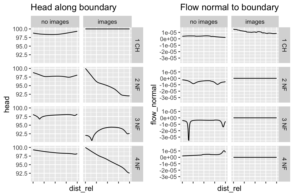
Finally, the function plot_bounds_behavior also includes the raw data of head and flow used to create the above plots (bounds_behavior$bounds_behavior), as well as a summary of these values which includes mean head on each of the boundaries and mean flow as the mean of the absolute value of flow normal to each boundary (bounds_behavior$table). To numerically check that the boundaries are working as expected, we can print bounds_behavior$table:
| bound | Mean flow, images | Mean flow, no images | Mean head, images | Mean head, no images |
|---|---|---|---|---|
| 1 CH | 1.07e-05 | 3.9e-06 | 100.00000 | 98.64171 |
| 2 NF | 0.00e+00 | 5.4e-06 | 95.01699 | 97.82476 |
| 3 NF | 0.00e+00 | 5.7e-06 | 93.32580 | 97.81516 |
| 4 NF | 0.00e+00 | 4.2e-06 | 96.37611 | 98.55836 |
Defining recharge / background flow
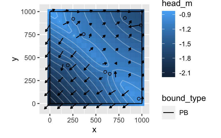
Background flow is parameterized by defining “recharge” in the aquifer. Recharge can be defined as a constant flow (F) or a recharge divide (D). In both cases, flow is defined as m3 / m-s, in the direction of the recharge vector. Recharge is therefore defined by specifying:
- Type of recharge: constant flow (F) or recharge divide (D)
- Recharge vector, pointing in the direction of flow
- Flow magnitude, in units of m3 / m-s
- Coordinates where the undisturbed water table (no wells) has a hydraulic head equal to aquifer$h0.
See ?define_recharge for more details.
# Define recharge for type "D"
recharge_params <- list(recharge_type="D",recharge_vector=c(500,500,501,501),
                        flow_main=1e-3,flow_opp=2e-3,x0=0,y0=0)

# Define bounds as "PB" -- pervious bounds, which have no effect (other than to define output grid)
bounds_recharge <- define_bounds(data.frame(bound_type=rep("PB",4),m=c(Inf,0,Inf,0),b=c(0,0,1000,1000)))
aquifer_recharge <- define_aquifer("confined",1,h0=0,z0=1,n=0.35,recharge=recharge_params,bounds=bounds_recharge)
gridded_2 <- get_gridded_hydrodynamics(wells_actual,aquifer_recharge,c(20,20),c(8,8))
The results can then be plotted, just as above:
Particle tracking
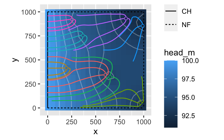
The package implements particle tracking in two ways: (1) tracking individual particles using track_particles and (2) estimating capture zones of wells using get_capture_zone, which initializes particles in the vicinity of wells and tracks them in reverse. Here we use get_capture_zone on the previous aquifer to generate particle tracking away from wells.
# wells <- wells
# wells[4,"Q"] <- 0.25
well_particles <- get_capture_zone(wells,aquifer_unconfined,t_max=365,n_particles=4)
gridded_3 <- get_gridded_hydrodynamics(wells,aquifer_unconfined)
ggplot() +
  geom_raster(data=gridded_1$head,aes(x,y,fill=head_m)) +
  geom_contour(data=gridded_1$head,aes(x,y,z=head_m),color="white",alpha=0.3) +
  geom_segment(data=aquifer_unconfined$bounds,aes(x1,y1,xend=x2,yend=y2,linetype=bound_type)) +
  geom_path(data=well_particles,aes(x,y,group=i,color=as.factor(wID)),show.legend = FALSE) +
  geom_point(data=wells_actual,aes(x,y,color=as.factor(wID)),shape=21,show.legend = FALSE) +
  coord_equal()
Integrating with anem-app
The basic functionality of this package is implemented in a Shiny application, which can be run by calling anem_app() or accessed online at shinyapps.io. The Shiny application provides an GUI for setting aquifer properties, drawing boundaries, defining recharge, adding wells, and tracking particles. It also displays results directly in the app. You can also download scenarios created on anem-app and import them into R. To do so, check out ?import_app_rds from this package to learn more.