Groundwater model

library(nitratesgame)

library(dplyr)
library(tidyr)
library(sf) # needed for package to represent well capture polygons
library(units) # needed for package, ensures proper units
library(ggforce) # for plotting axes with units
library(patchwork) # for aligning axes of multiple subplots

First we set some basic parameters for the scenario including:

Household water use
Seepage rate
- Annual precipitation
- Seepage fraction
Seepage fraction
Well source area
- radius of source area
Housing density

# Get area of hh withdrawal
# hh_annual <- set_units(76, "gallon/day") %>% # from USGS water data
#   set_units("ft^3/year") * 4
# precip_annual <- set_units(1070, "mm / year") #%>%
# seepage_fraction <- 0.4
# seepage_annual <- precip_annual * seepage_fraction
# area_of_withdrawal <- hh_annual / seepage_annual

# wells are screened from 10 ft to 20 ft depth below the water table
z1 <- set_units(10,"ft")
z2 <- set_units(20,"ft")

rs <- set_units(20, "ft") # this is the radius of the region of well capture
density <- set_units(0.5, "1/acre") # the housing density

Now we need a grid of septic systems. You can create an array of wells yourself or use get_hh_grid. The inputs to get_hh_grid are density and area as units objects.

area <- set_units(64, "acre")
hh_array <- get_hh_grid(density, area)
hh_array$id <- 1:nrow(hh_array) # supply an id

The groundwater model predicts the probability that a point source will contaminate at least one well in an array of wells. However, in this case we are interested in the probability that an array of septic fields (considered point sources) will lead to contamination in a single well. This problem can be modeled using get_intersection_probability by considering the well as a point source and the septic systems as “virtual wells” such that the spatial relationship between a well and septic system (point source) is the same as the relationship between the virtual well and well (now considered the point source). The function get_septic_well_array does this job for us. See the ?get_septic_well_array for details.

virtual_well_array <- get_septic_well_array(hh_array, "septic", z_range = c(z1, z2), rs = rs)

Here you can see that the virtual well array is identical to the septic array but rotated by 180 degrees around the origin.

library(ggplot2)
library(ggforce) # needed to plot axes using units objects
ggplot(mapping = aes(x, y, color = id)) +
  geom_point(data = hh_array, aes(shape = "septic systems"), size = 4, stroke = 1) +
  geom_point(data = virtual_well_array, aes(shape = "virtual wells"), size = 2) +
  scale_shape_manual(values = c(1, 16)) +
  scale_color_viridis_c(option = "B") + coord_equal()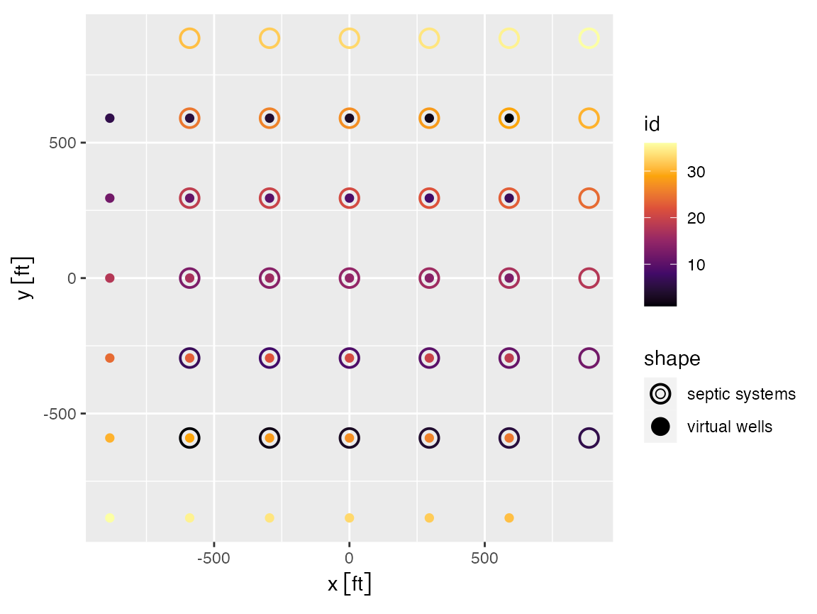

The array virtual_well_array contains sf geometries for each of the wells in \(\theta-\phi\) space. We can plot these geometries projected onto the z-axis such that it appears as viewed from the point source at the land surface. To do so we can take \(z_{projected}=\sin(\phi)\) and plot using geom_rect from ggplot. We zoom in only on \(\theta \in [0,pi/2]\).

p_wells <- ggplot(virtual_well_array) + 
  geom_rect(aes(xmin = theta1, xmax = theta2, ymin = sin(phi1), ymax = sin(phi2), fill = id), color = NA, alpha = 1) +
  scale_fill_viridis_c("id") +
  scale_y_reverse("sin(phi)") + 
  scale_x_continuous(breaks = c(0, pi/2), labels = c("0", "pi/2")) +
  coord_cartesian(xlim = c(0, pi/2))

p_phi <- ggplot(data.frame(alpha = seq(0,20,by=.1)) %>% dplyr::mutate(phi = atan(1/alpha))) + 
  stat_density(aes(sin(phi))) +
  scale_x_reverse("sin(phi)") + 
  coord_flip()
p_wells + p_phi + patchwork::plot_layout(widths=c(0.8,0.2))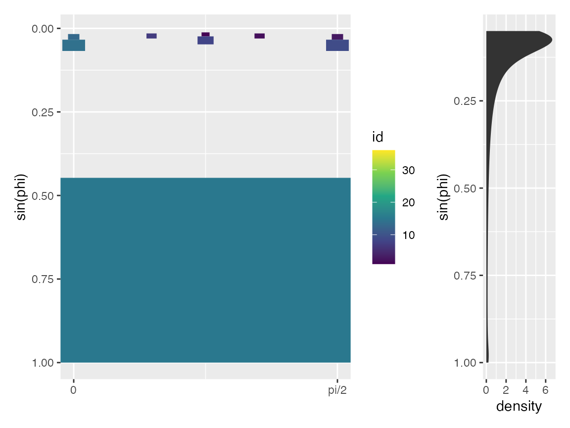

Get probability

Now get the probability of contamination of the well, using the virtual well array.

gw_example <- virtual_well_array %>%
  get_intersection_probability(theta_range = c(0,pi/2), alpha_range = c(0, 20),
                               self_treat = FALSE, show_progress = FALSE)
gw_example
#> [1] 0.1225776

Get multiple probabilities at once

Now, let’s get probabilities for each row of a tibble which contains columns for all of the appropriate input variables. Note that this must be a tibble and not a data.frame, because it has to store complex objects (i.e., list columns).

# Create a single row with constant parameters
params_row <- tibble(
  z1 = set_units(10, "ft"),
  z2 = set_units(20, "ft"),
  area = set_units(64, "acre"),
  theta_range = list(c(0, pi/4)), # this will be unlisted in the function
  alpha_range = list(c(0, 20)), # this will be unlisted in the function
  hh_array_type = "septic")

# Add varying parameters
params_df <- params_row %>%
  crossing(density = set_units(c(0, 0.5), "1/acre"), 
           rs = set_units(c(10, 20),"ft"), 
           self_treat = c(TRUE, FALSE)) # if self_treat is TRUE, a household cannot contaminate its own well

# Get probabilities
params_df$probs <- get_contamination_probabilities(params_df)
params_df[,c("density", "rs", "self_treat", "probs")]
#> # A tibble: 8 × 4
#>    density   rs self_treat  probs
#>   [1/acre] [ft] <lgl>       <dbl>
#> 1      0     10 FALSE      0.05  
#> 2      0     10 TRUE       0     
#> 3      0     20 FALSE      0.1   
#> 4      0     20 TRUE       0     
#> 5      0.5   10 FALSE      0.0613
#> 6      0.5   10 TRUE       0.0113
#> 7      0.5   20 FALSE      0.123 
#> 8      0.5   20 TRUE       0.0226