Identify-blind-spots • isw

library(isw)
#> Loading required package: expint
#> Loading required package: units
#> udunits database from /Library/Frameworks/R.framework/Versions/4.4-arm64/Resources/library/units/share/udunits/udunits2.xml

library(patchwork)
library(units)
library(png)
library(dplyr)
#> 
#> Attaching package: 'dplyr'
#> The following objects are masked from 'package:stats':
#> 
#>     filter, lag
#> The following objects are masked from 'package:base':
#> 
#>     intersect, setdiff, setequal, union
library(ggplot2)
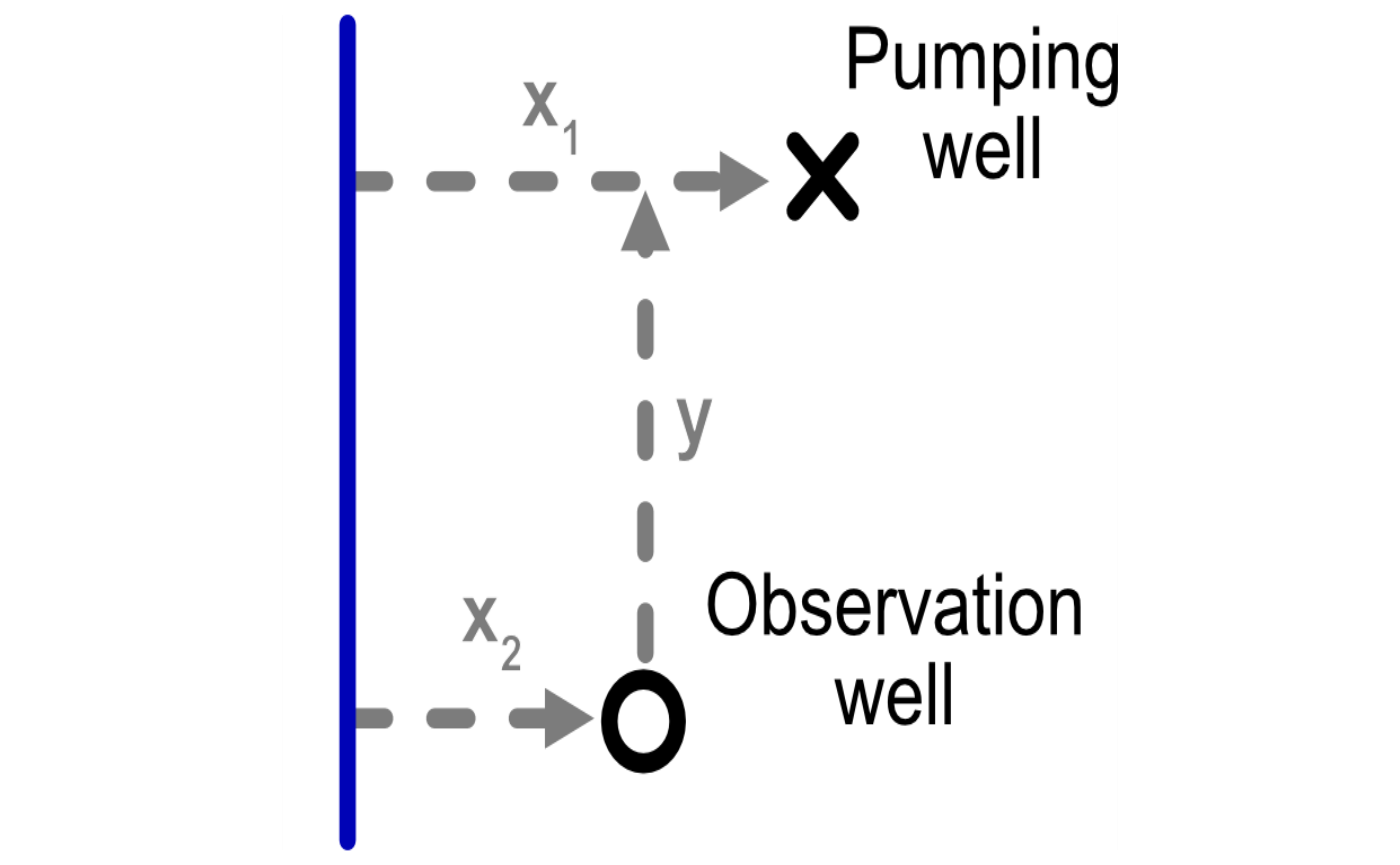
library(tidyr)

The package handles the configuration between river, pumping well, and observation well in a particular way, as shown in the figure below. We need to keep track of the following variables:

x1: Distance from the pumping well to the river
x2: Distance from the observation well to the river
y: Component of the distance between the two wells that is parallel to the river

We also need to consider aquifer parameters. We parameterize an aquifer with the following characteristics, based on the Glover paper:

Saturated thickness (D): 100 ft
Permeability (K): 0.001 ft/sec
Drainable porosity of the aquifer (V): 0.2

# example from Glover
# x1 <- set_units(c(1, 5, 10, 25, 50) * 1e3, 'ft')
D <- set_units(100, 'ft')
K <- set_units(0.001, 'ft/sec')
# t_sec <- set_units(1, "year") # sec in a year
V <- 0.2

Prepare themes for plotting

To make the plots look nice, we can create the following themes.

txt_size <- 16
theme_basic <- theme(
  line = element_line(size = 1, color = "black"), 
  panel.background = element_rect(fill = "white"), 
  legend.text = element_text(size = txt_size*0.9, color = "black"), 
  axis.title.x = element_text(size = txt_size, colour = "black"), 
  axis.title.y = element_text(size = txt_size, angle = 90, colour = "black"), 
  legend.title = element_text(size = txt_size, color = "black"))
#> Warning: The `size` argument of `element_line()` is deprecated as of ggplot2 3.4.0.
#> ℹ Please use the `linewidth` argument instead.
#> This warning is displayed once every 8 hours.
#> Call `lifecycle::last_lifecycle_warnings()` to see where this warning was
#> generated.


theme_std <- theme_basic %+replace% theme(
  panel.border = element_rect(fill = NA, colour = "black", size = 1), 
  panel.grid.major = element_blank(), 
  panel.grid.minor = element_blank(), axis.line = element_blank(), 
  axis.ticks.x = element_line(colour = "black", size = 0.5), 
  axis.ticks.y = element_line(colour = "black", size = 0.5), 
  axis.ticks.length = unit(1, "mm"), 
  axis.text.x = element_text(size = txt_size*0.9, colour = "black"), 
  axis.text.y = element_text(size = txt_size*0.9,  colour = "black", hjust = 1))
#> Warning: The `size` argument of `element_rect()` is deprecated as of ggplot2 3.4.0.
#> ℹ Please use the `linewidth` argument instead.
#> This warning is displayed once every 8 hours.
#> Call `lifecycle::last_lifecycle_warnings()` to see where this warning was
#> generated.

theme_diagram <- theme_basic %+replace% 
  theme(
  panel.border = element_rect(fill = NA, colour = NA, size = 1), 
  panel.grid.major = element_blank(), 
  panel.grid.minor = element_blank(), 
  axis.line = element_blank(), 
  axis.ticks.x = element_blank() , 
  axis.ticks.y = element_blank(), 
  axis.ticks.length = unit(1, "mm"), 
  axis.text.x = element_blank(), 
  axis.text.y = element_blank(), 
  axis.title.x = element_blank(), 
  axis.title.y = element_blank()) %+replace%
  theme(legend.position = c(0.8, 0.75), legend.box = 'vertical', legend.title = element_blank())
#> Warning: A numeric `legend.position` argument in `theme()` was deprecated in ggplot2
#> 3.5.0.
#> ℹ Please use the `legend.position.inside` argument of `theme()` instead.
#> This warning is displayed once every 8 hours.
#> Call `lifecycle::last_lifecycle_warnings()` to see where this warning was
#> generated.

Set up grid of locations

We first generate a tibble of different permutations of distances among the river, pumping well, and observation well.

# Pumping well locations
x1_coords <- seq(-1, 6, by = 0.05)
y1_coords <- seq(-1, 11, by = 0.2)
# x1_coords <- seq(0, 5, by = 0.05)
# y1_coords <- seq(0, 10, by = 0.2)
pump_wells <- crossing(x1 = x1_coords, y1 = y1_coords) %>%
  mutate(keep = x1 > 0 & x1 <= 5 & y1 >= 0 & y1 <=10,
         across(all_of(c("x1","y1")), function(x) set_units(x,"mi")))

# Observation well locations
x2_coords <- c(0.8, 1.6, 1, 3, 4)
y2_coords <- c(2, 4, 8.5, 1, 6)
well_diam <- set_units(50, "ft")

# Times
t_years <- 5 #c(0.05, seq(0.1,5, by = 0.1))
  
obs_wells <- tibble(x2 = x2_coords, y2 = y2_coords, well_diam) %>%
  mutate(`Obs. well` = as.factor(row_number()),
         across(all_of(c("x2","y2")), function(x) set_units(x,"mi")))

wells <- crossing(pump_wells,
                  obs_wells,
                  t = set_units(t_years,'year')) %>%
  mutate(K = K, D = D, V = V,
         y = abs(y2 - y1),
         id = row_number())



# locations <- tribble(~x1, ~y, ~`Obs. well`, ~`Pumping well`,
#                      0.2, 1.5, "a", "c",
#                      0.8, 1.5, "a", "d",
#                      0.2, 0, "b", "c",
#                      0.8, 0, "b", "d") %>%
#   mutate(x2 = 0.5,
#          across(all_of(c("x1","x2","y")), function(x) set_units(x,"mi")), id = row_number())

To visualize these permutations we can plot them.

p_grid <- ggplot() + 
  geom_point(data = pump_wells, aes(x1, y1), size = 0.5) + 
  geom_point(data = pump_wells %>% filter(!keep), aes(x1, y1), size = 0.5, color = "red") + 
  geom_point(data = obs_wells, aes(x2, y2, shape = `Obs. well`, color = `Obs. well`), size = 4) + 
  # scale_shape_manual(values = c(0, 5)) +
  xlab("Distance from river (x)") + 
  ylab("Distance along river (y)") +
  # scale_color_discrete("Well type") + 
  theme_std +
  coord_equal()
p_grid
#> Warning: The `scale_name` argument of `continuous_scale()` is deprecated as of ggplot2
#> 3.5.0.
#> This warning is displayed once every 8 hours.
#> Call `lifecycle::last_lifecycle_warnings()` to see where this warning was
#> generated.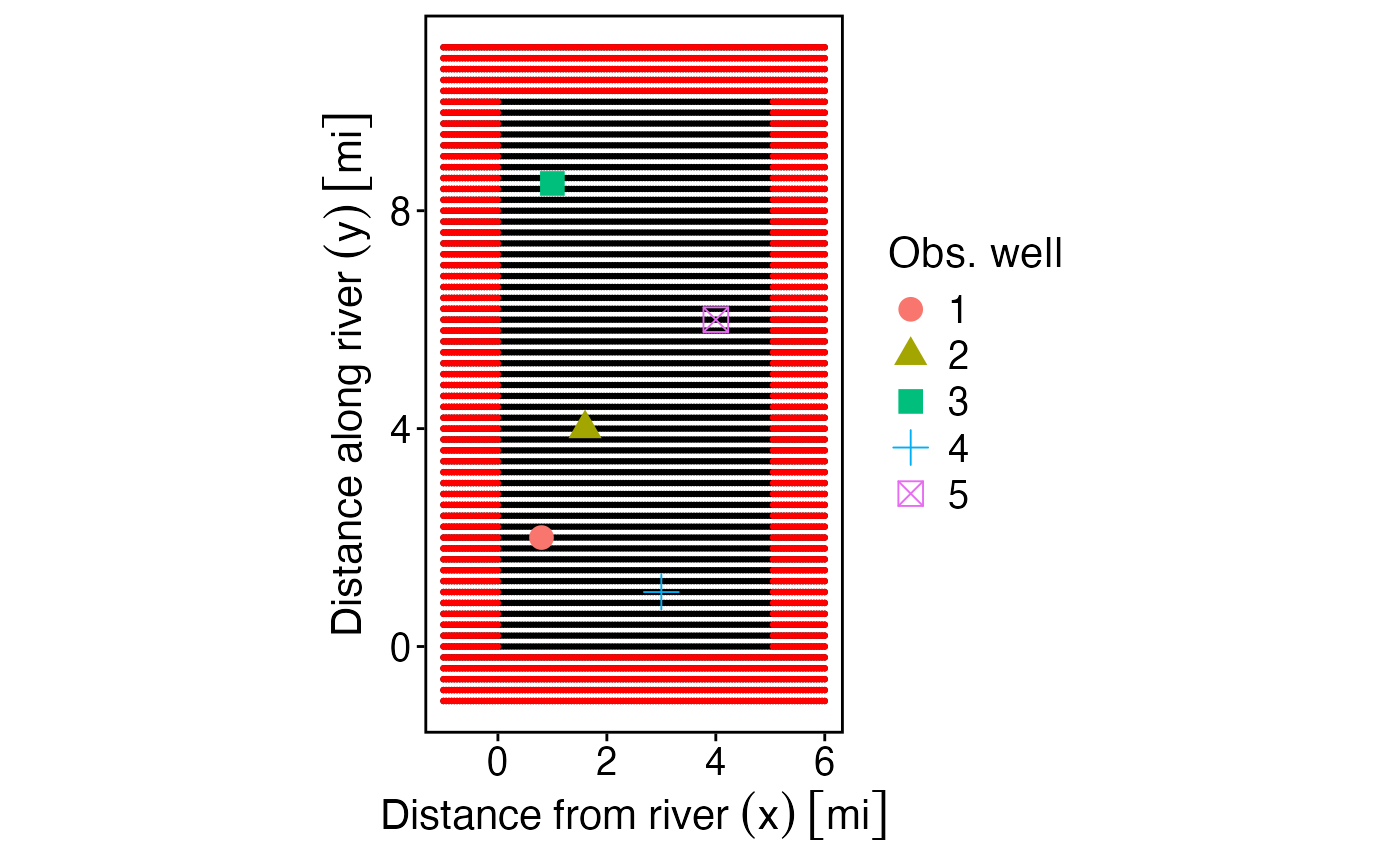

Now we can get aquifer depletion with the get_depletion_from_pumping function. As seen in the output, the function returns a data.frame with two columns:

stream_depletion_fraction: The fraction of pumping at that timestep that is associated with stream depletion (opposed to drawing down the aquifer)
aquifer_drawdown_ratio: The amount of aquifer drawdown (i.e., change in groundwater level) per unit pumping.

depletion <- get_depletion_from_pumping(wells %>% mutate(x1=abs(x1)))
head(depletion)
#>   stream_depletion_fraction aquifer_drawdown_ratio
#> 1                 0.6742365 -9.519514e-02 [s/ft^2]
#> 2                 0.6742365 -1.003251e-05 [s/ft^2]
#> 3                 0.6742365 -1.471024e-02 [s/ft^2]
#> 4                 0.6742365 -2.396764e-01 [s/ft^2]
#> 5                 0.6742365 -6.351577e-04 [s/ft^2]
#> 6                 0.6742365 -1.187152e-01 [s/ft^2]

We can now add the depletion to the tibble to the original data frame for plotting and analysis.

df_abline <- crossing(slope = c(1,2,4), intercept = 0)
wells_calcs <- wells %>%
  bind_cols(as_tibble(depletion)) %>%
  mutate(ratio = -stream_depletion_fraction / aquifer_drawdown_ratio,
         ratio_cut = cut(ratio, c(0, df_abline$slope, Inf)))
head(wells_calcs)
#> # A tibble: 6 × 17
#>     x1   y1 keep    x2   y2 well_diam `Obs. well`      t      K    D     V
#>   [mi] [mi] <lgl> [mi] [mi]      [ft] <fct>       [year] [ft/s] [ft] <dbl>
#> 1   -1 -1   FALSE  0.8  2          50 1                5  0.001  100   0.2
#> 2   -1 -1   FALSE  1    8.5        50 3                5  0.001  100   0.2
#> 3   -1 -1   FALSE  1.6  4          50 2                5  0.001  100   0.2
#> 4   -1 -1   FALSE  3    1          50 4                5  0.001  100   0.2
#> 5   -1 -1   FALSE  4    6          50 5                5  0.001  100   0.2
#> 6   -1 -0.8 FALSE  0.8  2          50 1                5  0.001  100   0.2
#> # ℹ 6 more variables: y [mi], id <int>, stream_depletion_fraction <dbl>,
#> #   aquifer_drawdown_ratio [s/ft^2], ratio [ft^2/s], ratio_cut <fct>

p_ratio <- ggplot(wells_calcs %>% group_by(x1, y1) %>% filter(ratio == min(ratio), keep)) + 
  geom_point(aes(as.numeric(abs(aquifer_drawdown_ratio)), as.numeric(stream_depletion_fraction), alpha = as.numeric(x1), color = ratio_cut)) +
  geom_abline(data = df_abline, aes(slope = slope, intercept = intercept)) +
  geom_abline(data = df_abline[df_abline$slope==1,], aes(slope = slope, intercept = intercept),color="red",size=1) +
  scale_color_viridis_d("Stream depletion (cfs)\nper aquifer drawdown (ft)")+
  scale_alpha_continuous("Distance\nfrom river",range = c(1, 0.2)) +
  guides(color = "none") +
  theme_std +
  scale_x_continuous("Aquifer drawdown per cfs pumping (ft)", limits=c(0, 3)) + 
  scale_y_continuous("Stream depletion per cfs pumping (cfs)", limits = c(0,1), breaks = seq(0,1,by = 0.2))
#> Warning: Using `size` aesthetic for lines was deprecated in ggplot2 3.4.0.
#> ℹ Please use `linewidth` instead.
#> This warning is displayed once every 8 hours.
#> Call `lifecycle::last_lifecycle_warnings()` to see where this warning was
#> generated.
p_ratio
#> Warning: Removed 154 rows containing missing values or values outside the scale range
#> (`geom_point()`).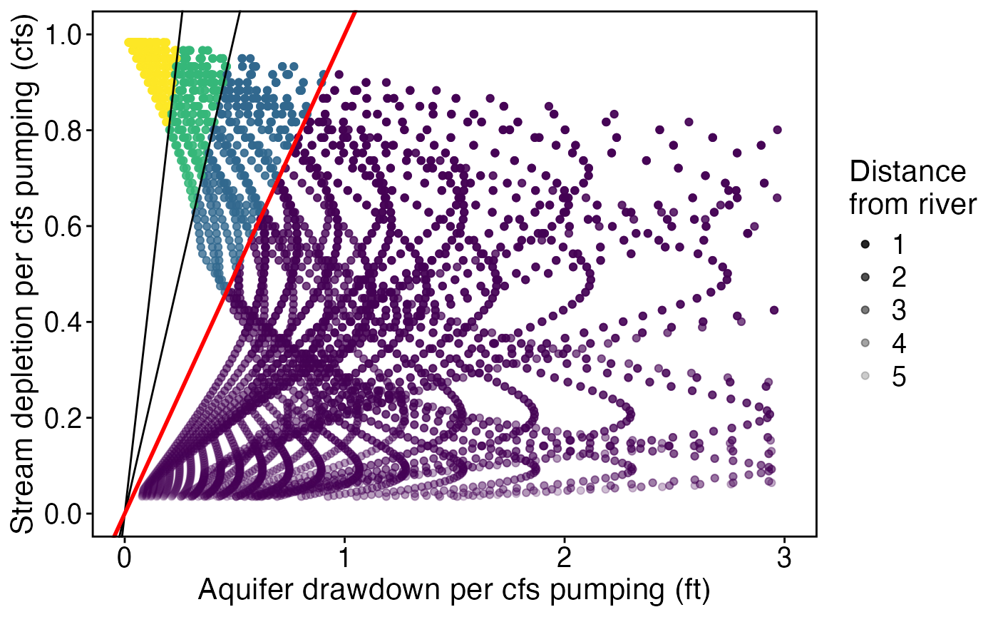

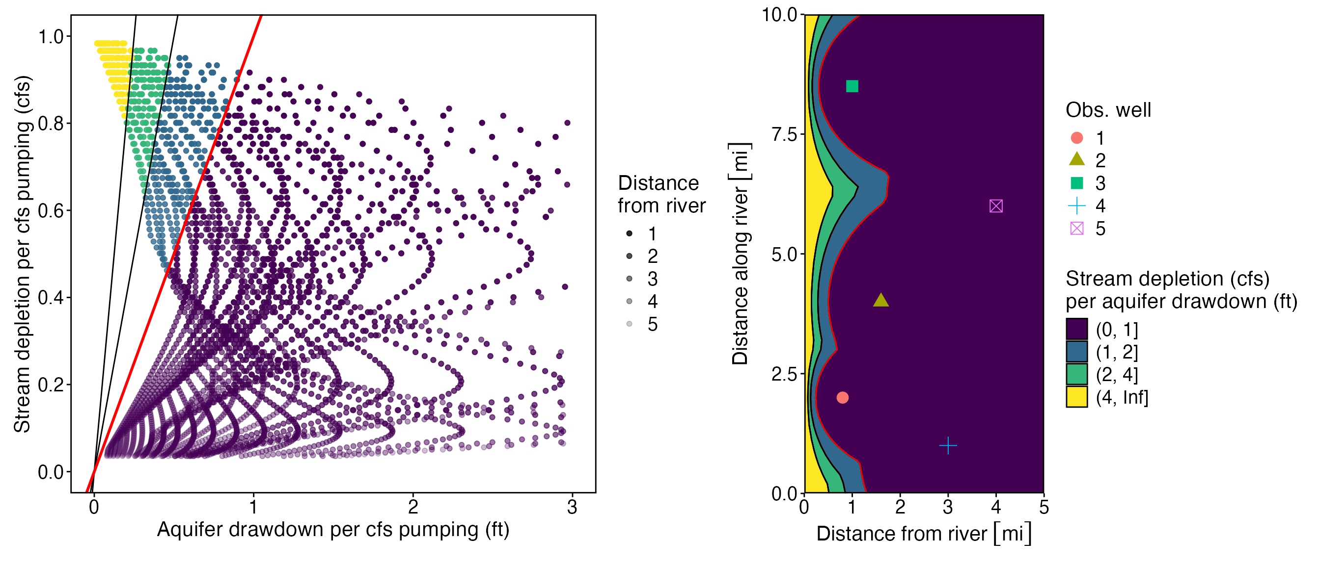
Now let’s plot the same ratio as a map

wells_calcs_ratio <- wells_calcs %>% 
  group_by(x1, y1) %>% filter(ratio == min(ratio)) %>%
  mutate(ratio = as.numeric(ratio),
         blind_spot = as.numeric(ratio) > 2)

p_blind_spot<- ggplot(wells_calcs_ratio %>% group_by(x1, y1) %>% filter(ratio == min(ratio))) + 
  # geom_contour_filled(aes(x1, y1, z = as.numeric(ratio)), breaks = c(0,1,2,4, Inf)) +
  geom_contour_filled(aes(x1, y1, z = as.numeric(ratio)), breaks = c(0,1,2,4, Inf), color = "black") +
  geom_contour(aes(x1, y1, z = as.numeric(ratio)), breaks = c(1,2), color = "red") +
  geom_contour(aes(x1, y1, z = as.numeric(ratio)), breaks = c(0,2,4, Inf), color = "black") +
  geom_point(data = obs_wells, aes(x2, y2, shape = `Obs. well`, color = `Obs. well`), size = 4) + 
  scale_fill_viridis_d("Stream depletion (cfs)\nper aquifer drawdown (ft)") +
  scale_x_units("Distance from river") +
  ylab("Distance along river") +
  theme_std +#%+replace% 
  # theme(
  #   panel.margin = unit(c(0, 0, 0, 0), "null"),
  #   plot.margin = unit(c(0, 0, 0, 0), "null")) +
  coord_equal(xlim = c(0,5),ylim = c(0,10),expand=FALSE)
p_blind_spot
#> Warning: Contour data has duplicated x, y coordinates.
#> ℹ 244 duplicated rows have been dropped.
#> Warning: Removed 61 rows containing non-finite outside the scale range
#> (`stat_contour_filled()`).
#> Warning: Contour data has duplicated x, y coordinates.
#> ℹ 244 duplicated rows have been dropped.
#> Warning: Removed 61 rows containing non-finite outside the scale range
#> (`stat_contour()`).
#> Warning: Contour data has duplicated x, y coordinates.
#> ℹ 244 duplicated rows have been dropped.
#> Warning: Removed 61 rows containing non-finite outside the scale range
#> (`stat_contour()`).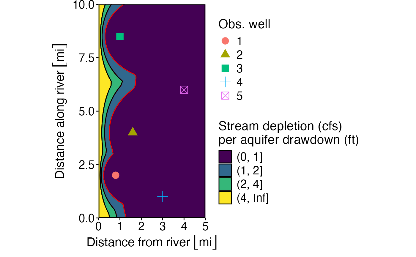

p_ratio + p_blind_spot
#> Warning: Removed 154 rows containing missing values or values outside the scale range
#> (`geom_point()`).
#> Warning: Contour data has duplicated x, y coordinates.
#> ℹ 244 duplicated rows have been dropped.
#> Warning: Removed 61 rows containing non-finite outside the scale range
#> (`stat_contour_filled()`).
#> Warning: Contour data has duplicated x, y coordinates.
#> ℹ 244 duplicated rows have been dropped.
#> Warning: Removed 61 rows containing non-finite outside the scale range
#> (`stat_contour()`).
#> Warning: Contour data has duplicated x, y coordinates.
#> ℹ 244 duplicated rows have been dropped.
#> Warning: Removed 61 rows containing non-finite outside the scale range
#> (`stat_contour()`).