Getting started with ISW package

This vignette illustrates key elements of the isw package, used to generate simple models of interconnected surface water. The package includes functions to estimate stream depletion and aquifer drawdown.

The idealized model in isw assumes the wells are screened over the saturated thickness of the aquifer, the stream fully penetrates the aquifer, all flow is horizontal, and the transmissivity is uniform and insensitive to changes in water level.

The package can be installed using remotes::install_github("gopalpenny/isw"), and loaded as:

library(isw)

Main package functions

The isw package has three primary functions to understand interconnected surface waters:

• get_stream_depletion_fraction: Estimate stream depletion due to pumping well(s)
• get_aquifer_drawdown_ratio: Estimate aquifer drawdown due to pumping well(s) (no stream)
• get_depletion_from_pumping: Estimate stream depletion and aquifer drawdown (with stream)

We’ll see how each of these works, below. Note that within these models, representation of the stream uses the method of well images, which basically says that streams with constant head can be modeled by mirroring wells across the stream and switching the sign of pumping. In other words, a pumping well and and injection well on opposite sides of the stream will ensure constant hydraulic head at the midpoint between the two wells, assuming the rates of pumping and injection are equal in magnitude.

Note that the get_aquifer_drawdown_ratio does not assume a stream, and therefore works only for a single well. Both get_stream_depletion_fraction and get_depletion_from_pumping account for an image well on the other side of the stream.

Aquifer parameters

Aquifers in isw are represented with just a few variables. Let’s consider an aquifer with the following characteristics:

• Saturated thickness (D): 100 ft
• Permeability (K): 0.001 ft/sec
• Drainable porosity of the aquifer (V): 0.2

Note that isw uses the units package to keep track of dimensionality, therefore we can begin by loading this package. The set_units function can be used to specify units objects, and therefore aquifer parameters.

library(units)
D <- set_units(100, "ft")
K <- set_units(0.001, "ft/sec")
t <- set_units(5, "year")
V <- 0.2 # unitless

Some basic calculations

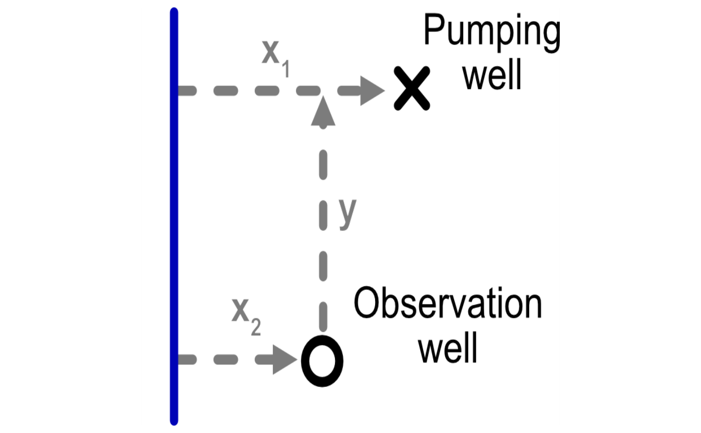
The main functions in isw use variables to describe the spatial relationship among pumping wells, observation wells, and the river. These include the following variables illustrated in the figure below:

• x1: distance from the stream to a pumping well,
• x2: distance from the stream to a observation well well, and
• y: distance between observation and pumping wells parallel to the river.

Note that the stream can be omitted by specifying x1 = Inf and x2 = Inf.

Estimating stream depletion

The get_stream_depletion_fraction() function estimates stream depletion at time t as a fraction of pumping from an individual pumping well, following Glover and Balmer (1954). We can call get_stream_depletion_fraction by specifying x1, the aquifer parameters, and the elapsed time t since pumping initiated.

x1 <- set_units(0.5, "mi")
stream_depletion_fraction <- get_stream_depletion_fraction(x1 = x1, K = K, D = D, V = V, t = t)
stream_depletion_fraction
#> [1] 0.8335347

We can get total stream depletion by multiplying this fraction by a pumping rate, for instance 1 cfs:

pumping_rate <- set_units(1, "ft^3/s")
stream_depletion <- stream_depletion_fraction * pumping_rate
stream_depletion
#> 0.8335347 [ft^3/s]

As can be seen, the stream depletion fraction is simply the percentage of total pumping, at time t, that is coming from stream depletion. Or put another way, it is:

$$\text{stream depletion fraction (at time t)} = \frac{\text{rate of stream depletion (at time t)}}{\text{rate of pumping (at time t)}}$$

Estimating aquifer drawdown

The get_aquifer_drawdown_ratio() function gives the change in water level per unit pumping at an observation well (without a stream). The parameters x1, x2, and y specify the geometry of the pumping well, observation well, and stream.

y <- set_units(1, "mi")
aquifer_drawdown_ratio <- get_aquifer_drawdown_ratio(y = y, x1 = Inf, x2 = Inf, K = K, D = D, V = V, t = t)
aquifer_drawdown_ratio
#> -1.540413 [s/ft^2]

Note that get_aquifer_drawdown_ratio has an optional parameter, well_diam that defaults to a value of 0. When specified, drawdown does not increase inside the well. In other words, when r<well_diam/2, drawdown is calculated as if r=well_diam/2, where r is the distance between the pumping and observation wells ($r = \sqrt{(x_2 - x_1)^2 + y^2}$).

Depletion and drawdown

The get_depletion_from_pumping() function estimates stream depletion fraction (using get_stream_depletion_fraction) and changes in water level at an observation well (get_aquifer_drawdown_ratio) due to abstraction from a pumping well at time t after pumping initiates. Like get_stream_depletion_fraction, and unlike get_aquifer_drawdown_ratio, the function accounts for a the effect of the stream as a constant head boundary using, as noted above, the method of images.

This function uses a couple new parameters. The x2 parameter ($x_2$) is the distance between the observation well and the stream. If r is the distance between the pumping and observation wells, y is the component of this distance that is parallel to the stream. In other words, $r^2 = (x_2-x_1)^2 + y^2$. Keeping the remaining parameters the same as before, we can call this function as:

x2 <- set_units(1e3, "ft")
y <- set_units(1e3, "ft")
depletion_from_pumping <- get_depletion_from_pumping(x1 = x1,
                                                     x2 = x2,
                                                     y = y,
                                                     K = K,
                                                     D = D,
                                                     V = V,
                                                     t = t)
depletion_from_pumping
#>   stream_depletion_fraction aquifer_drawdown_ratio
#> 1                 0.8335347     -1.049005 [s/ft^2]

Parameter combinations with vector and data.frame objects

We can also estimate drawdown at multiple distances from a pumping well. We use the function get_aquifer_drawdown_ratio, noting that both stream_depletion_fraction and get_depletion_from_pumping also allow multiple parameter combinations specified as vector or data.frame objects. Let’s get this ratio a distances ranging from 1 ft to 10 miles, after 2 years of pumping.

y <- set_units(seq(1/5280, 10, length.out = 200), "mi")
t <- set_units(2, 'year')
aquifer_drawdown_ratio <- get_aquifer_drawdown_ratio(y = y, x1 = Inf, x2 = Inf, K = K, D = D, V = V, t = t)
head(aquifer_drawdown_ratio)
#> Units: [s/ft^2]
#> [1] -14.384728  -5.496842  -4.397988  -3.755887  -3.301625  -2.950755

Equivalently, we can specify parameter combinations in a data.frame. The tidyr function crossing() can be very helpful to get multiple parameter combinations.

library(tidyr)

# create tibble with all parameter combinations
df <- tibble(K = K, D = D, V = V, t = t, x1 = Inf, x2 = Inf) %>%
  crossing(y = set_units(seq(1/5280, 10, length.out = 200), "mi"))

# call function with tibble to specify parameters
aquifer_drawdown_ratio <- get_aquifer_drawdown_ratio(df)
head(aquifer_drawdown_ratio)
#> Units: [s/ft^2]
#> [1] -14.384728  -5.496842  -4.397988  -3.755887  -3.301625  -2.950755

For simplicity, let’s assume the well was pumping 1 cusec over those two years. The change in water level is calculated as aquifer_drawdown_ratio multiplied by the pumping rate.

pumping_rate <- set_units(1, "ft^3/sec")
aquifer_drawdown <- aquifer_drawdown_ratio * pumping_rate

We can then plot the drawdown as a function of pumping using ggplot. The bind_cols function from dplyr allows us to join the drawdown results with the original data.frame.

library(ggplot2)
library(dplyr)
drawdown_df <- df %>% 
  bind_cols(drawdown = aquifer_drawdown)

ggplot(drawdown_df, aes(y, drawdown)) +
  geom_line()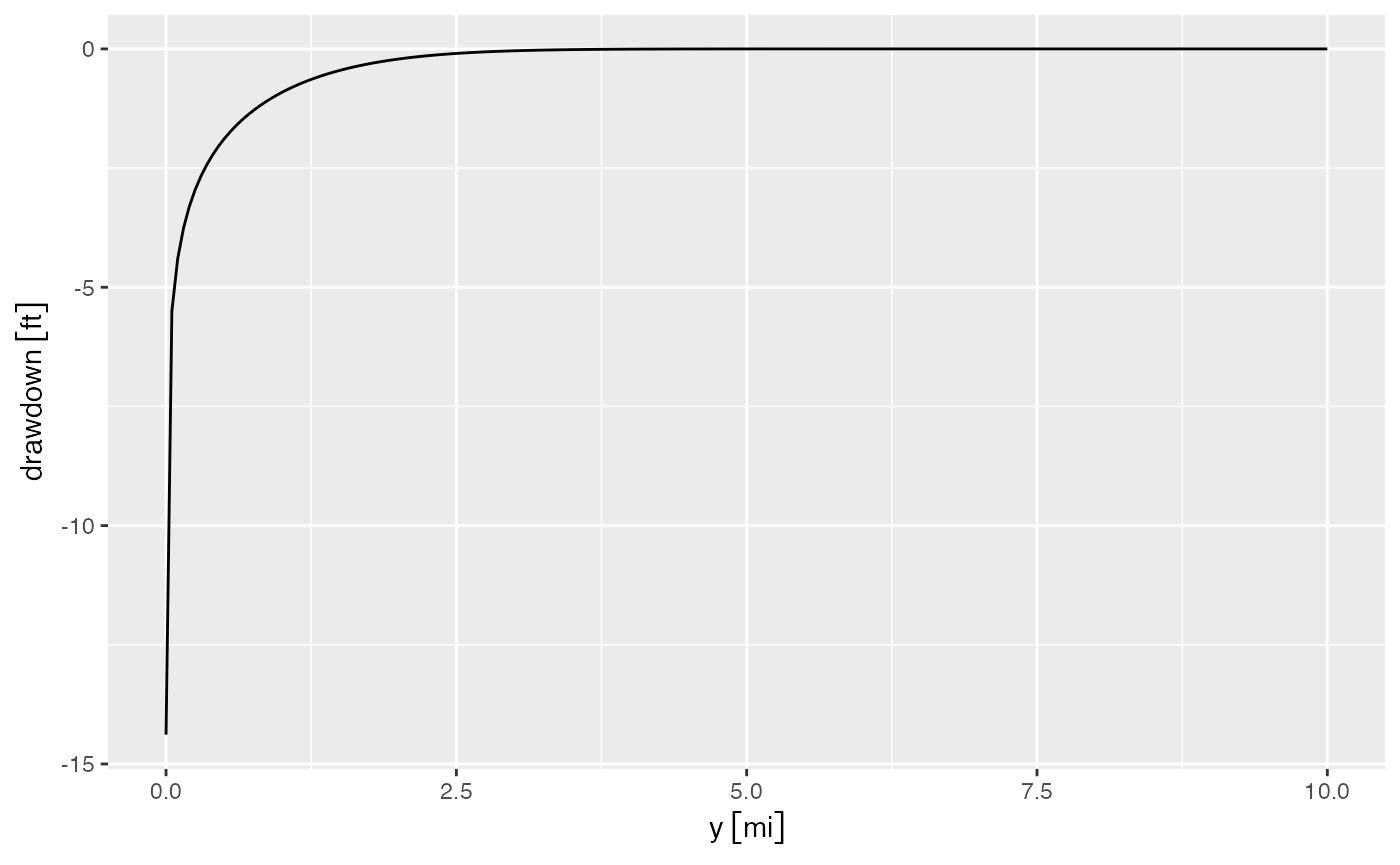

Checking the drawdown calculations

As a check, to give confidence in this calculation, we can calculate the volume of water drained from the aquifer as drawdown times the drainable porosity for circular bands (with differential radius $dr$) around the well. For simplicity, we use the dplyr::mutate function to calculate this value.

dy <- y[2] - y[1]
drawdown_df <- drawdown_df %>% 
  mutate(d_area = dy * 2 * pi * y,
         volumetric_drawdown = drawdown * d_area * V)

In an aquifer with no recharge, the total volumetric drawdown should be equal to the pumping rate over the time period, 1 cusec over five years or 63 million ft³. The water drained from the aquifer can be calculated using sum(volumetric_drawdown), which gives a result of -63 million ft³.

The total radial flow towards the well can be calculated as $q = 2 \pi r D K \frac{\partial h}{\partial r}$ (the typical negative sign in Darcy’s law is removed because we are calculating flow in the direction of negative r). We can run this calculation and plot flow towards the aquifer.

drawdown_df <- drawdown_df %>% 
  mutate(flow_towards_well = 2 * pi * y * D * K * (drawdown - lag(drawdown)) / dy,
         flow_towards_well = set_units(flow_towards_well, "ft^3/s"))

ggplot(drawdown_df, aes(y, flow_towards_well)) + geom_line() +
  geom_abline(slope = 0, intercept = 1, color = "red", linetype = "dashed")
#> Warning: Removed 1 row containing missing values or values outside the scale range
#> (`geom_line()`).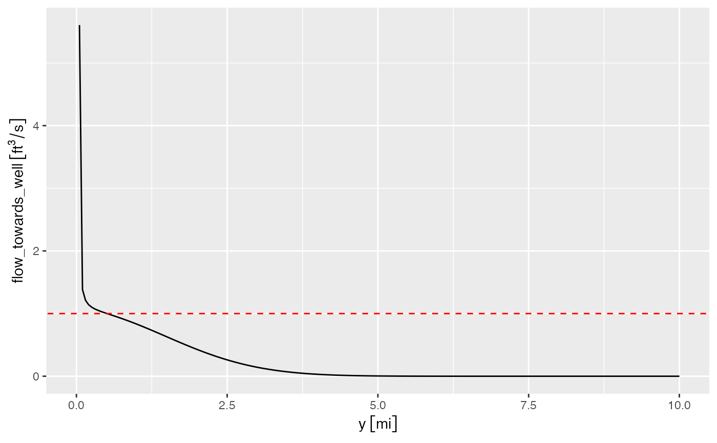

Note that closer to the pumping well this calculation suffers from coarse discretization of the domain causing the flowrate to diverge from 1 ft³/s. You can verify this yourself by, for instance, changing the radius to y <- set_units(seq(1, 5, length.out = 200), "ft") and re-running the calculations.

References

Glover, Robert E., and Glenn G. Balmer. “River Depletion Resulting from Pumping a Well near a River.” Eos, Transactions American Geophysical Union 35, no. 3 (1954): 468–70. https://doi.org/10.1029/TR035i003p00468.